Introduction
In autonomous driving, prediction is a measure of the future behavior of “agents” on the road. This typically includes behaviors (such as “lane following”, “turning left”, “turning right”), coupled with predicted trajectories consisting of (x, y) coordiantes. These predictions are then used by the Autonomous Vehicle’s (AV’s) planning and decision making modules, to ensure safe and optimal maneuvers that avoid collisions — for example, if a vehicle is predicted to come into the AV’s lane, the AV should respond accordingly by slowing down and allowing them to enter. The prediction problem can be complex, as scenes on the road can evolve very uniquely depending on the context such as number of agents on the road, road features, weather conditions, and so on. Additionally, the AV’s own behaviors affect the agents around it that predictions are sought for.
There is a plenty of literature proposing solutions to the traffic prediction problem using neural networks ([1], [2], [3] and many others) or probabilistic graphical models ([4], [5] and many others). However, I have not come across any work on solving it using Mixture Density Networks.
Mixture Density Networks (MDNs) [6], which I covered in a previous blog post, are neural networks that output the parameters of a mixture model, such as a Gaussian Mixture Model. MDNs are useful for tasks where a given input can potentially produce multiple outputs according to some probability. My post on MDNs shows the iconic toy problem where given an x coordinate, there could be multiple y coordinates. For example, given x=0.25, y could be {0, 0.5, 1} with perhaps equal probability of 1/3, 1/3, 1/3 per y coordinate. If such a problem is solved with neural networks trained with Mean Squared Error to produce a singular y output, it will likely only lead to the average y values — in the example aforementioned, y=0.5 for x=0.25.

The above example extends to traffic prediction very naturally. Let’s set up an example scene to explain why. An agent (a vehicle we are predicting for) approaches a Y-split in the road, and can go either right, or left. Depending on the agent’s past trajectory, perhaps one of the two options has a higher probability, though either is still probable up to a certain point. In this case, say we train a neural network regressor at this specific Y-split on past data of cars flowing through, using Mean Squared Error, to output a singular trajectory.
We can frame the inputs at timestep t as a series of (x, y) coordinates representing the past trajectory of the agent up to some P timesteps in the past, thus [latex]X_t = \{ (x_{t-P}, y_{t-P}), (x_{t-P+1}, y_{t-P+1}), …, (x_t, y_t) \}[/latex]. And the ouputs, the prediction, can be the agent’s trajectory up to some time horizon H in the future again consisting of coordinates at each timestep, thus [latex]Y_t = \{ (x_{t+1}, y_{t+1}), (x_{t+2}, y_{t+2}), …, (x_{t+H}, y_{t+H}) \}[/latex].
Take the scenario of traffic at a Y-split where agents can either go right or left with a 50/50 probability (up to a certain point before the Y-split) given a similar past trajectory. And say we have a balanced dataset of examples of these. Again, as seen in the toy example above, the Neural Network regressor trained with Mean Squared Error or the like, will end up giving an average of the two possible future trajectories, as depicted below. The image on the left shows the typical trajectories agents can take at this scene, and the image on the right shows the likely output trajectory of a vanilla neural network regressor trained on this scene.


As seen above, traffic scene prediction is a good candidate for where Mixture Density Networks can be used. In traffic scene prediction, we need a distribution over behaviors an agent can exhibit — for example, an agent could turn left, turn right, or go straight. Thus, Mixture Density Networks can be used to represent “behaviors” in each of the mixture it learns, where the behavior consists of a probability and trajectory ((x, y) coordinates up to some time horizon in the future). In the autonomous driving domain, it is helpful to have not just the predictions (the trajectories of agents around an autonomous vehicle), but the uncertainty attached to predictions, for better planning and decision making. A Mixture Density Network is a good candidate here additionally, as it will output a mixture of behaviors that have a probability (certainty) attached to each along with a standard deviation over the trajectories.
Problem Definition
In autonomous driving, data is typically gathered by the perception module, which consists of reading and logging sensors such as through video cameras, LiDaR, Radar, and so on. These sensors are meant to perceive the world and the state around the Autonomous Vehicle (AV), which include perceiving other agents on the road (vehicles, pedestrians, etc). In prediction (and other modules in the AV), raw sensor data such as images or point clouds can be used as input. Though I’ve read prediction papers where this raw data is used as input, a landmark paper by Waymo points to a number of papers that “show the brittleness of using raw sensor data” for learning to drive by means of prediction and planning [1] . Thus, some alternate pre-processing of raw sensor data is necessary. This data can be used to feed through neural network based object detectors, and a tracking module that uses perhaps the likes of Kalman filters to create traces of other agents on the road — individual agents tracked over time, using numeric representations of their dimensions (the size of the agent in meters, for example), position as a (x, y) coordinate, heading, velocity, and so on. Additionally, an HD map of the current location which includes features of the environment such as lanes represented as a series of (x, y) coordinates, can be used to place the perceived agents in the scene around the AV.

Where work on traffic prediction by Waymo [1], Uber [2], and others [3], create an intermediate rasterized (image) representation using this pre-processed data to feed to a convolutional network, I propose keeping it simple and feeding these numbers directly into a neural network without an intermediate representation expressed as an image. Thus, the input, [latex]X[/latex] can consists of a series of vectors representing the past positions (past trajectory) up to the current timestep, heading at the current timestep, and velocity at the current timestep, of individual agents in the scene. These inputs can be mapped to outputs, [latex]Y[/latex] — predictions of where the agents will be in some future time horizon such in the next 2 to 8 seconds from the present moment (their future trajectory).
Context is paramount in traffic prediction. For example, you observe a cyclist in a dedicated bike lane on a road going straight. And you also observe a vehicle stopped in the bike lane some distance ahead of the cyclist. Without taking the stopped vehicle into account, you would likely not be able to predict that the cyclist will have to pass the stopped vehicle by leaving the bike lane and coming into the vehicle traffic lanes. Thus, context must include other agents that may or may not affect a particular agent we are predicting for. Features of the current scene also provide important context, that must be taken into account. For example, the contours of the lane (if they curve right, an agent following the lane will need to adjust accordingly), locations and states of traffic lights (traffic light is red, so agents will likely stop as they approach), traffic rules (one way roads, etc), and so on.
For the traffic prediction problem, I propose a single feedforward neural network that at a given timestep [latex]t[/latex] can take up to some [latex]N[/latex] agents as inputs (their past trajectories up to some [latex]t-P[/latex] timesteps) and produce [latex]N-1[/latex] outputs for predictions of their future trajectories up to some time horizon [latex]t+H[/latex]. The [latex]N[/latex] agents include the ego vehicle (the AV), as the position and movement of the ego vehicle itself may affect other agents around it and can provide context for predictions for the others, and then [latex]N-1[/latex] of the closest agents to the ego based on euclidean distance, as predictions for irrelevant agents such as those much further away than the AV are not necessary. This consolidated input will provide multi-agent context to the network, allowing it to learn interactions among agents and how that relates to predictions of their future trajectories. The outputs need only include the trajectories of the [latex]N-1[/latex] closest agents, as we need not predict for the AV.
More specifically, at a given timestep [latex]t[/latex], the input for each agent, [latex]X[/latex], can include their past trajectory of (x, y) coordinates up to some [latex]P[/latex] previous timesteps, their heading, their velocity, and additionally I propose the lane contours of the lane they are currently in expressed as (x, y) coordinates. Thus, for each agent [latex]n[/latex], [latex]X^n_t = \{ (x_{t-P}, y_{t-P}), (x_{t-P+1}, y_{t-P+1}), …, (x_t, y_t), heading_t, veolcity_t, (x^{lane}_1, y^{lane}_1), (x^{lane}_2, y^{lane}_2), …, (x^{lane}_?, y^{lane}_?) \}[/latex]. The outputs for each agent [latex]n[/latex] includes their trajectory up to some future time horizon [latex]H[/latex], thus [latex]Y^n_t = \{ (x_{t+1}, y_{t+1}), (x_{t+2}, y_{t+2}), …, (x_{t+H}, y_{t+H}) \}[/latex]. Following these, the full input to the neural network at a single timestep would be the ego-centric (from the perspective of the AV) “scene” [latex]I_{t} = \{ X^1_t, X^2_t, …, X^N_t \}[/latex] and full output would be [latex]O_{t} = \{ Y^1_t, Y^2_t, …, Y^{N-1}_t \}[/latex]. Note that in order to make this a feasible and somewhat consistent (“normalized”) problem for the neural network to learn, all euclidean (x, y) coordinates can be made relevant to the AV’s current position at the current timestep. That is, setting [latex](x^0_{t=0}, y^0_{t=0}) = (0.0, 0.0)[/latex], and having all other coordinates of all agents trajectory positions and lane contours offset relatively.
As a simple feedforward neural network (as opposed to a more complex LSTM setup) will be used, unfortunately the input and output sizes will need to be fixed. This is somewhat problematic because we have to know up front how many agents are in a given scene, and additionally, how many behaviors we want the MDN to predict (as in, number of mixtures — more on that below). For example, if the network is trained using input that includes the ego vehicle plus the 9 closest agents, but only 3 other agents are observed. However, this can be overcome as we can zero-pad all inputs and outputs if none are available at any given timestep. In the aforementioned example, all inputs and outputs for the additional agents can just consist of all 0’s.
Mixture Density Network Setup
As a MDN is being used for this problem, the neural network does not output [latex]O_{t}[/latex] directly. Instead, it outputs a set of mixture coefficients (probabilities attached to each mixture) [latex]\alpha[/latex], means [latex]\mu[/latex], and standard deviations [latex]\sigma[/latex] — the parameters of a Gaussian Mixture Model (GMM). These parameters can then be sampled from to get [latex]O_{t}[/latex] for predicted future trajectories for the individual agents, which are used along with the uncertainty of each trajectory expressed as a probability and standard deviation of the trajectory, to feed into the AV’s planning module.
While the MDN can be framed to output a Gaussian mixture, [latex]\{\alpha^{1:K}_t, \mu^{1:K}_t, \sigma^{1:K}_t \}[/latex] where [latex]K[/latex] is the number of desired mixtures, for each individual (x, y) euclidean coordinate in the trajectory, it can instead be biased to learn behaviors in the mixtures. Instead of making every point a mixture, we can move the mixture to a higher level where the mixture represents a set of (x, y) coordinates — the trajectory — as a whole, and thus, map to a certain behavior. In this setup, each “behavior” is intended to represent a high-level behavior an agent on the road could exhibit, such as “go left”, “go right”, “go straight”, and so on.
We can represent behaviors as [latex]B^{1:K}_t[/latex], where [latex]K[/latex] is the number of mixtures output for the GMM being represented by the MDN. Each behavior [latex]B^k_t[/latex] can have a coefficient [latex]\alpha^{k}_{t}[/latex] representing the probability of the likelihood of that mixture, so [latex]\sum_{k=1}^{K} \alpha^k_t = 1[/latex]. Additionally, each behavior contains a set of (x, y) coordinates up to a time horizon [latex]H[/latex] represented as means [latex]M^k_t = (\mu^{x, k}_{t+1:t+H}, \mu^{y, k}_{t+1:t+H})[/latex], to produce the predicted trajectory defined earlier: [latex]Y_t = \{ (x_{t+1}, y_{t+1}), (x_{t+1}, y_{t+1}), …, (x_{t+H}, y_{t+H}) \}[/latex]. For the standard deviation [latex]\sigma[/latex], it can be taken per (x, y) coordinate as a whole, rather than individually for each x and each y. The standard deviation then represents the uncertainty of the coordinate as a whole — so per behavior [latex]k[/latex], in [latex]K[/latex] total behaviors, we have [latex]S^k_t = \sigma^{k}_{t+1:t+H}[/latex].
The predicted behaviors per agent per timestep [latex]t[/latex] can be represented as [latex]B^k_t = \{\alpha^k_t, M^k_t, S^k_t\}[/latex]. If for our MDN we have [latex]N[/latex] agents as input — the ego vehicle (the AV) and [latex]N-1[/latex] closest agents in euclidean distance — the desired outputs include predicted behavior of the N-1 closest agents. The full output [latex]O_t[/latex] of the neural network in the MDN is then [latex]\{ B^{1, 1:K}_t, B^{2, 1:K}_t, …, B^{N-1, 1:K}_t \}[/latex].

The number of mixtures (the number of behaviors) is an open question, and will likely require some thought and experimentation. However, a good starting point would be 3, simply based on the intuition that in traffic, a vehicle can go left, right, or straight. Left or right could mean switch lanes or a full left or right turn, which the network should learn based on the usual behavior and lane contours in the scene.
[2]’s approach to traffic prediction involves using a neural network outputting a single behavior for an agent as a trajectory of (x, y) coordinates up to some future time horizon. Additionally, they output a standard deviation per each (x, y) coordinate in the trajectory. [2] find empirically that training such a network requires curriculum, where the network is first trained with the Mean Displacement Error, and then the standard deviation outputs are trained. Note that the Mean Displacement Error simply involves taking the mean of the euclidean distance of each point in the predicted trajectory with the ground truth trajectory. The equations for calculating the Mean Displacement Error, and the half-Gaussian loss including the standard deviation can be seen in the figure below.

The MDN can be trained similarly via curriculum where first the network is trained with Mean Displacement Error, where the means ([latex]mu[/latex]’s) of the (x, y) coordinates output for each mixture for each agent are trained, and then the full outputs including the standard deviation’s ([latex]\sigma[/latex]’s) are trained using the half-Gaussian distribution loss. The main difference is that we need to train additionally for multiple outputs (behaviors/mixtures) per individual agent, and thus also train the MDN coefficients [latex]\alpha[/latex]’s. This can simply be done by taking a softmax of the coefficients and multiplying them with the mean loss for each mixture, and then taking the sum of the loss across all mixtures. That is, [latex]L_{total} = \sum_{k=1}^{K} \alpha^k L_{ij}[/latex] where [latex]L_{ij}[/latex] are the losses either from equation (2) or (5) displayed from [1]’s approach, depending on which part of the curriculum is being trained.
Additionally, as this is a complex problem for the network to learn, I propose applying another curriculum to the training by progressively training for the number of agents in the output starting from number of trainable agents = 1. Meaning, first train the mixtures output for the first agent (agent 1) only, by a) using Mean Displacement Error first and b) full half-Gaussian second, and then training the first two agents together (agents 1 and 2) similarly, and so on up to all agents in the full output.
Code for this loss function in Python, using Chainer, is displayed below. The input variable holds the full input at some timestep as mentioned earlier (past trajectories and lane contours of an ego vehicle and its closest [latex]N-1[/latex] agents). The num_agents represents the total number of agents in the inputs and outputs. trainable_agents represents the number of agents in the curriculum being currently trained for as described earlier (1, 1:2, 1:3, 1:4, …, 1:N-1). And finally output holds the ground truth trajectory of (x, y) coordinates for each agent being predicted for, up to future some time horizon.
coef, mu, ln_var = self.fprop(input)

coef = coef.reshape(output.shape[0], num_agents, num_mixtures)
coef = F.softmax(coef, axis=2)
mu = F.reshape(mu, (output.shape[0], num_agents, num_mixtures, -1, 2))
ln_var = F.reshape(ln_var, (output.shape[0], num_agents, num_mixtures, -1))

output = output.reshape(output.shape[0], num_agents, 1, -1, 2)
output = F.repeat(output, num_mixtures, 2)

coef = coef[:, :trainable_agents, :]
ln_var = ln_var[:, :trainable_agents, :, :]

x_true = output[:, :trainable_agents, :, :, 0]
y_true = output[:, :trainable_agents, :, :, 1]
x_pred = mu[:, :trainable_agents, :, :, 0]
y_pred = mu[:, :trainable_agents, :, :, 1]

if curriculum_step == 1:
    loss = F.sum(coef * F.sum(((x_true-x_pred)**2) + ((y_true-y_pred)**2), axis=3))
else:
    displacement_sq = ((x_true-x_pred)**2) + ((y_true-y_pred)**2)
    ln_var = F.clip(ln_var, -300., 300.) #Numerical stability
    var = F.exp(ln_var)
    loss = F.sum(coef * F.sum(((displacement_sq/(2*var)) + F.log(F.sqrt(2 * math.pi * var))), axis=3))
Data
The data can originate from either sensors on an AV driving around, or fixed CCTV style cameras pointed at a road. In either case, it will be necessary to track agents in the scene at a given moment with an identifier, and preprocess the sensor or video footage into “traces” — a vector of (x, y) coordinates observed for the agent’s position over time, expressed in a particular reference system, as the agents enter and exit the vicinity of the AV or fixed camera.
These traces can then be divided into inputs and outputs to form a dataset in the following manner. As an example setup, if an agent is seen for a total of 15 seconds at a frame rate of 25 Hz, that gives us 375 total observed positions of the agent over time. If we set the prediction time horizon (referenced as [latex]H[/latex] previously) to 2 seconds at 25 Hz (thus 50 future positions desired for prediction), based on an input of the past 1 second of the agent’s past positions (25 past positions), our inputs and outputs can be divided from the total 375 frames available for the agent, for every timestep [latex]t \in \{0:325\}[/latex]. At each timestep [latex]t[/latex], the dataset for this agent can contain input = [latex]\{(x_{t-25}, y_{t-25}), …, (x_t, y_t)\}[/latex] and output = [latex]\{(x_{t+1}, y_{t+1}), …, (x_{t+50}, y_{t+50})\}[/latex]. At timestep [latex]t = 0[/latex], as positions are not available from the previous 1 second for the agent, the input can be zero-filled.
Additionally, for adding in the environmental context, an HD map of the locations the agent traces are collected from will be required. This map can provide the lane contours for each agent for the inputs.
All data for inputs, outputs, and lane contours, should be ego-centered. Meaning, for the ego vehicle in the input, the current (x, y) position at [latex]t=0[/latex] would be (0.0, 0.0), and all other (x, y) positions should be relative to this, to normalize the data for the neural network.
Results
Experiments were performed on a proprietary dataset consisting of 24 hours of detection at a fixed scene, using the following setup and hyperparameters:
| Parameter | Setting |
| Number of mixtures | 3 |
| Past positions of agents, P | 1 second = 25 |
| Time horizon for prediction, H | 2 seconds = 50 |
| Ego vehicle + number of closest agents | 1+9 = 10 |
| Distance to find closest agents | 40 meters |
| Number of layers | 10 |
| Hidden units | 1024 |
| Activations | ReLU |
The dataset was split into train, validation and test sets. After curriculum training the MDN as described above to a point where satisfactory results were achieved on the validation set, predictions on the test set were compared against the ground truths using Root Mean Squared Error (RMSE), using the Manhattan distance between the coordiantes. This RMSE was compared to an implementation of DESIRE [3], which was trained and tested on the same dataset.
While DESIRE achieved an RMSE of 0.38979 on the test set, the MDN achieved an RMSE of 0.401587, when testing only the first agent’s output. When testing all 9 agent’s outputs against the ground truths, the MDN achieved an RMSE of 0.478878 (when using the trajectory from the most likely behavior). Note that with DESIRE, only a single agent’s prediction is tested at a time. Furthermore, DESIRE constitutes a series of complex LSTMs with several expensive intermediate steps, whereas the MDN can achieve similar results for multiple agents at a time, in a single forward pass with a simpler feedforward network.
Upon inspecting the results in detail, I also noticed that the mixtures were appropriately mapping to plausible high-level behaviors with adequate probabilities given the agent’s history, particularly in situations where there was ambiguity in where the agent could go next. I also observed in many cases the probability being almost 1 ([latex]\alpha=1[/latex]) for a behavior for agents where the network strongly expressed they could only go in a certain direction given their past trajectory. Otherwise, the performance and learning of the behaviors will require more quantitative experiments to measure, as the definition and ground truths of behavior are harder to measure as opposed to raw predicted trajectories being compared using RMSE.
Conclusions
For the traffic prediction problem, Mixture Density Networks (MDN) can be used to learn a distribution over agents’ trajectories in a traffic scene. If the MDN is framed to produce a full trajectory within each Gaussian mixture as a whole, as opposed to framing each point in the trajectory to be a mixture in its own, the MDN can be biased to learn higher-level behaviors of agents, leading to more accurate and plausible predictions. These behaviors come with a probabilities at the behavior level, and standard deviation over the trajectory predictions, allowing for uncertainty-aware decision making in the Autonomous Vehicle context.
This method can achieve similar prediction accuracy to state-of-the-art methods such as DESIRE [3], when measuring the Root Mean Squared Error of the Manhattan distance of the predicted coordinates in the trajectories to the ground truths. While state-of-the art methods may require series of complex neural networks such as LSTMs, with expensive intermediate processing steps, the MDN can achieve similar results for multiple agents at a time, in a single forward pass with a simple feedforward network, using no intermediate rasterized representation.
The limitations with this approach are that the number of agents being input and output, and the number of mixtures and thus behaviors, are fixed at train time. To overcome this limitation, perhaps in future work RNNs can be explored for feeding inputs and receiving outputs as sequences that are terminated with separator markers, similar to how the dataset is composed to train and test the Differentiable Neural Computer:
https://github.com/AdeelMufti/DifferentiableNeuralComputer. Furthermore, in future work, this method should be trained and tested on a variety of scenes, with an ablation study to determine how much the multi-agent and environmental context helps with prediction. The number of Gaussian mixtures also requires further consideration and experimentation.
References
[1] Mayank Bansal et al., ChauffeurNet: Learning to Drive
by Imitating the Best and Synthesizing the Worst, 2018, https://arxiv.org/abs/1812.03079.
[2] Nemanja Djuric et al., Short-term Motion Prediction of Traffic Actors for Autonomous Driving using Deep Convolutional Networks, 2018, https://arxiv.org/abs/1808.05819.
[3] Namhoon Lee et al., DESIRE: Distant Future Prediction in Dynamic Scenes with Interacting Agents, 2017, http://www.robots.ox.ac.uk/~tvg/publications/2017/CVPR17_DESIRE.pdf.
[4] Jens Schulz et al., Interaction-Aware Probabilistic Behavior Prediction in Urban Environments, 2018, https://arxiv.org/abs/1804.10467.
[5] Jingbo Zhou et al., R2-D2: a System to Support Probabilistic Path Prediction in Dynamic Environments via “Semi-Lazy” Learning, 2013, https://www.researchgate.net/publication/262271558_R2d2_A_System_to_Support_Probabilistic_Path_Prediction_in_Dynamic_Environments_via_semilazy_Learning.
[6] Christopher M. Bishop, Mixture Density Networks, 1994, https://publications.aston.ac.uk/373/1/NCRG_94_004.pdf.