Covariance Matrix Adaptation Evolution Strategy (CMA-ES) in Python

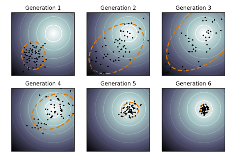
According to OpenAI, Evolution Strategies are a scalable alternative to Reinforcement Learning. Where Reinforcement Learning is a guess and check on the actions, Evolution Strategies are a guess and check on the model parameters themselves. A “population” of “mutations” to seed parameters is created, and all mutated parameters are checked for fitness, and the seed adjusted towards the mean of the fittest mutations. CMA-ES is a particular evolution strategy where the covariance matrix is adapted, to cast a wider net for the mutations, in an attempt to search for the solution.

To demonstrate, here is a toy problem. Consider a shifted Schaffer function with a global minimum (solution) at f(x=10,y=10):

[latex]f(x,y)=0.5+\frac{sin^{2}[(x-10)^{2}-(y-10)^{2}]-0.5}{[1+0.001[(x-10)^{2}+(y-10)^{2}]]^{2}},\ \ \ \ \ f(10,10)=0[/latex]

The fitness function F() for CMA-ES can be treated as the negative square error between the solution being tested, and the actual solution, against the Schaffer function:

[latex]F(s_1,s_2) = -(f(s_1,s_2) – f(10,10))^2[/latex]

Therefore, the task for CMA-ES is to find the solution [latex](s_1=10, s_2=10)[/latex]. Given the right population size [latex]\lambda[/latex] and the right [latex]\mu[/latex] for CMA-ES, it eventually converges to a solution. With [latex]\lambda=64[/latex] and [latex]\mu=0.25[/latex], a visualization of CMA-ES as it evolves a population over generations can be seen below.

The animation below depicts how CMA-ES creates populations of parameters that are tested against the fitness function. The blue dot represents the solution. The red dots the entire population being tested. And the green dot the mean of the population as it evolves, which eventually fits the solution. You see the “net” the algorithm casts (the covariance matrix) from which the population is sampled, is adapted as it is further or closer to the solution based on the fitness score.
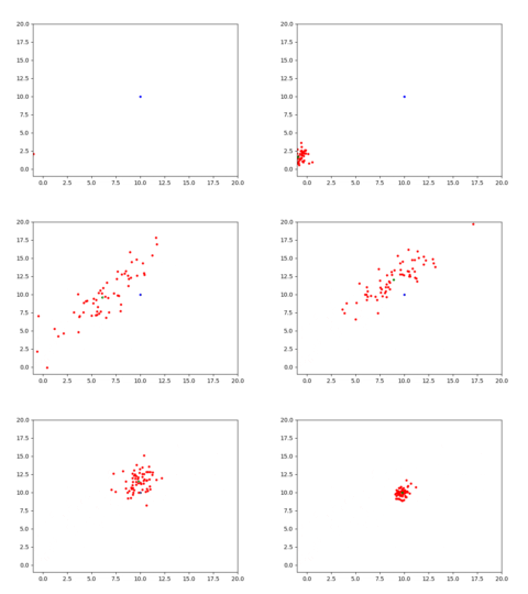
CMA-ES in action, quickly finding a solution to a shifted Schaffer function.

A simple (yet powerful) implementation for CMA-ES in Python, and this toy problem, is available at https://github.com/AdeelMufti/WorldModels/blob/master/toy/cma-es.py. I translated the (mu/mu_w, lambda)-CMA-ES algorithm to Python.

Mixture Density Networks in Chainer

There are excellent blog posts and guides available on Mixture Density Networks, so I will not try to replicate the effort. This post provides a quick summary, and implementation code in the Chainer deep learning framework.

In summary, Mixture Density Networks are Neural Networks that output the parameters of a Mixture Model, such as a Gaussian Mixture Model, instead of the desired output itself. The Mixture Model is then sampled from to get the final output. This is particularly useful when given a certain input, there could be multiple outputs based on some probability.

The outputs from the neural network, in the case of Gaussian Mixture Models, include a set of probabilities [latex]\alpha[/latex] (coefficients), set of means [latex]\mu[/latex], and set of standard deviations [latex]\sigma[/latex]. For example, if output is y given an x, and you choose to have 3 Gaussian mixtures, the output of your neural network would be: [latex]\alpha_1, \alpha_2, \alpha_3, \mu_1, \mu_2, \mu_2, \sigma_1, \sigma_2, \sigma_3[/latex]. The [latex]\alpha[/latex] sum to 1 and represent the probability of each mixture being the likely candidate, and the [latex]\mu[/latex] and [latex]\sigma[/latex] represent the distribution of y within the given mixture and can be used to sample y.

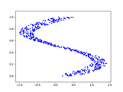
Take as a toy example consider the dataset of (x, y) coordinates represented in the graph below:

Toy dataset of (x, y) coordinates graphed.

The blue dots represent the desired y value given an x value. So at x=0.25, y could be {0, 0.5, 1} (roughly). In this case, training a neural network using Mean Squared Error to output y directly will cause the network to learn the average of the y values given x as inputs, as shown below (red dots represent y output from the neural network):

A neural network trained with Mean Squared Error produces an averaged output.

For this type of problem, a Mixture Density Network is perfectly suited. If trained properly, and sampled from enough times given all x values in the dataset, the Mixture Density Network produces the following y outputs. It better learns the distribution of the data:

A Mixture Density Network can learn the distribution of the data.

The output of the neural network is simply the number of dimensions in your output (1 in this example), times the number of desired mixtures, times 3 (the coefficient, mean, and standard distribution). In Chainer, a Linear layer can be used to output these numbers.

The loss function is essentially the negative log of the Gaussian equation multiplied by the softmax’d coefficients: [latex]-\ln\{\alpha\frac{1}{\sqrt{2\pi}\sigma}\exp{-\frac{(y-\mu)^2}{2\sigma^2}}\}[/latex], where [latex]\sum\alpha=1[/latex] [1]. This can be represented in Chainer easily as follows:

alpha = F.softmax(alpha)
density = F.sum(
    alpha *
    (1 / (np.sqrt(2 * np.pi) * F.sqrt(var))) *
    F.exp(-0.5 * F.square(y - mu) / var)
    , axis=1)
nll = -F.sum(F.log(density))

Full implementation of a Mixture Density Network in Chainer, for the toy problem shown above, can be found at: https://github.com/AdeelMufti/WorldModels/blob/master/toy/mdn.py

[1] Christopher M. Bishop, Mixture Density Networks (1994)