For this work I investigated the use of the DNC in the lifelong learning context. Lifelong learning differs from multi-task learning slightly. In multi-task learning, the goal is to learn multiple tasks simultaneously. In lifelong learning, the goal is to learn multiple tasks sequentially, without forgetting old tasks.
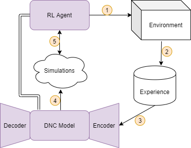
In the paper I introduced the Neural Computer Agent, where a model of the environment is learned by a DNC, and a paired agent is trained to maximize rewards using the Proximal Policy Optimization (PPO) algorithm in simulations generated by the DNC model.
Schematic for the iterative lifelong RL architecture, the Neural Computer Agent. An agent interacts with the environment to collect experience, which is used to train a predictive DNC model. The model is then used to simulate the environment to train the agent. The agent then rolls out to the environment again to collect new experience and iterate again.
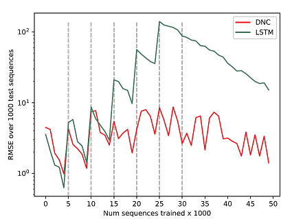
I hypothesized that the DNC can be used to learn a global model as opposed to task-specific local models which are used in multi-task and lifelong learning. I first tested the DNC on an integer addition task where the task progressively changed in difficulty, and found that the DNC can leverage past knowledge and adapt to new tasks quickly, outperforming LSTM by an order of magnitude. Additionally, the DNC continued to perform well on the prior learned integer addition tasks after it learned new ones.
DNC and LSTM performance over the course of training on multiple progressively difficult addition tasks. The curriculum steps switch at every 5, 000 sequences trained, until 30, 000 sequences, where the most difficult task remains fixed until training concludes.
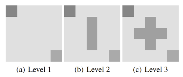
I tested The Neural Computer Agent on two toy RL environments that contained multiple tasks. I found that in both environments, the DNC was able to learn an adequate model of all tasks, and the Neural Computer Agent solved each environment iteratively entirely in simulations.
The levels (tasks) present in the Obstacle-Based Grid Navigation environment. The levels are designed to progressively increase in difficulty by adding obstacles. The agent starts at the top left cell of the grid, and has to reach the goal cell at the bottom right in a minimum number of steps.
Intrinsic Motivation is all the rage in Reinforcement Learning these days. In human psychology, intrinsic motivation refers to behavior that is driven by internal rewards. One example of intrinsic motivation is, if something new and usual is encountered, it may cause someone to give it more attention. In RL, a fine balance between exploration and exploitation is required. If exploration is inadequate, an agent may get stuck in a local optimum. This is particularly problematic if extrinsic rewards are sparse or not well defined. Thus, a mechanism for intrinsic motivation can be used to cause the agent to explore.
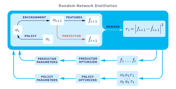
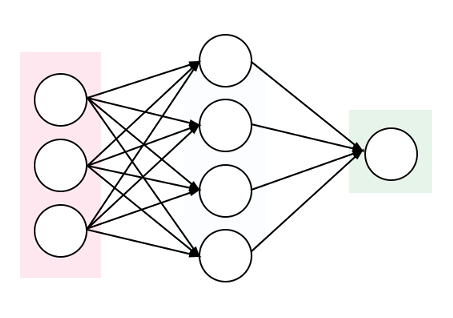
Enter Random Network Distillation (RND), as proposed by OpenAI: https://openai.com/blog/reinforcement-learning-with-prediction-based-rewards/. In summary, a randomly initialized network — the target — is used to distill another network — the predictor — by training the predictor to learn the output of the target network given all states encountered so far as input. The measure of error between the target network and predictor network, can be used as a metric for intrinsic motivation when training a RL agent. As the target network and predictor network process states they repeatedly see while the RL agent does rollouts in the environment, the predictor network learns the target network’s reaction to the states, and thus the intrinsic reward becomes increasingly lower as the same state is seen again and again. However, if a new state is encountered, the predictor network would not be aligned with the target network on the new state, thus producing a spike in the error and increase in intrinsic motivation, allowing the agent to explore the new state encountered due to the higher rewards.
I decided to create my own implementation in Chainer of a Proximal Policy Optimization (PPO) RL agent, to use intrinsic rewards through Random Network Distillation. I kept the implementation as close as possible to the details in OpenAI’s paper. The implementation can be seen at: https://github.com/AdeelMufti/RL-RND.
I conducted an experiment with PixelCopter-v0, which I’ve been dealing with as a baseline task for a series of experiments involving Reinforcement Learning, Evolution Strategies, and Differentiable Neural Computers. I’ve noted that for several learning algorithms (CMA-ES, PPO, Policy Gradients), the agent easily and quickly falls into a local optimum. It goes up a few times (action = up), and then after that all actions are “no action”, until it falls on the floor and the game is over. This allows it to get a higher score than with random actions, but after that it never improves. When experimenting with PPO with RND for intrinsic motivation, I turned off the external rewards. Very interestingly, the agent fell into that exact local optimum, simply based on the intrinsic rewards!
As I conduct more experiments and adjust my implementation, I will be updating this post.
For my MSc Artificial Intelligence at the University of Edinburgh, my dissertation included 4 months of research. I investigated the use of the Differentiable Neural Computer (DNC) for model-based Reinforcement Learning / Evolution Strategies. A predictive, probabilistic model of the environment was learned in a DNC, and used to train a controller in video gaming environments to maximize rewards (score).
The difference between Reinforcement Learning (RL) and Evolution Strategies (ES) are detailed here. However, in this post and my dissertation, the two are used interchangeably as either is used to accomplish the same goal — given an environment (MDP or partially observable MDP), learn to maximize the cumulative rewards in the environment. The focus is rather on learning a model of the environment, which can be queried while training an ES or RL agent.
The authors of the DNC conducted some simple RL experiments using the DNC, given coded states. However, to the best of my knowledge, this is the first time the DNC was used in learning a model of the environment entirely from pixels, in order to train a complex RL or ES agent. The experiments I conducted showed the DNC outperforming Long Short Term Memory (LSTM) used similarly to learn a model of the environment.
Learning a Model
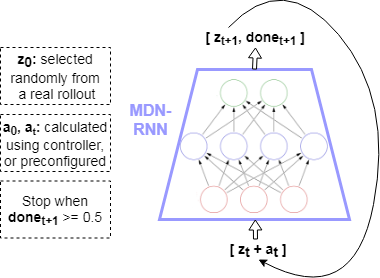
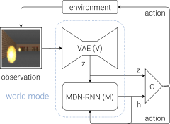
The model architecture is borrowed from the World Models framework (see my World Models implementation onGitHub). Given a state in an environment at timestep t, [latex]s_t[/latex], and an action [latex]a_t[/latex] performed at that state, the task of the model is to predict the next state [latex]s_{t+1}[/latex]. Thus the input to the model is [latex][s_t + a_t][/latex], which produces output (prediction) [latex]s_{t+1}[/latex]. Note that the states in this case consist of frames from the game at each timestep consisting of pixels. These states are compressed down to latent variables z using a Convolutional Variational Autoencoder (CVAE), therefore more specifically the model maps [latex][z_t + a_t] => z_{t+1}[/latex].
The model consists of a Recurrent Neural Network, such as LSTM, that outputs the parameters of a Mixture Density Model — in this cased, a mixture of Gaussians. This type of architecture is known as a Mixture Density Network (MDN), where a neural network is used to output the parameters of a Mixture Density Model. My blog post on MDNs goes into more details. When coupled with a Recurrent Neural Network (RNN), the architecture is known as MDN-RNN.
Thus, in learning a model of an environment, the output of the MDN-RNN “model” is not simply [latex]z_{t+1}[/latex], but the parameters of a Gaussian Mixture Model ([latex]\alpha, \mu, \sigma[/latex]) which are then used to sample the prediction of the next state [latex]z_{t+1}[/latex]. This allows the model to be more powerful by becoming probabilistic, and encode stochastic environments where the next state after a given state and action can be one of multiple.
For the experiments I conducted, the architecture of the model used a DNC where the RNN is used in World Models, thus, the model is composed of a MDN-DNC. Simply, the recurrent layers used in the MDN are replaced with a DNC (which itself contains recurrent layers that are additionally coupled with external memory).
The hypothesis was that using the DNC instead of vanilla RNNs such as LSTM, will allow for a more robust and algorithmic model of the environment to be learned, thus allowing the agent to perform better. This would particularly be true in complex environments with long term dependencies (meaning, a state perhaps hundreds or thousands of timesteps ago needs to be kept in context for another state down the line).
Experiments And Results
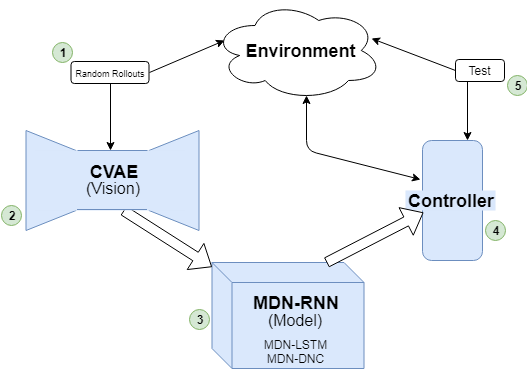
Experimentation schematic, based on the World Models framework.
The model of the environment learned is then used to train an RL agent. More specifically, features from the model are used, and in the case of the World Models framework, this consists of the hidden and cell states [latex]h_t, c_t[/latex] of the LSTM layers of the model at every timestep. These “features” of the model, coupled with the compressed latent representation of the environment state, z, at a given timestep t is used as input to a controller. Thus, the controller takes as input [latex][z_t + h_t + c_t][/latex] to output action [latex]a_t[/latex] to be taken to achieve a high reward. CMA-ES (more details in my blog post on CMA-ES in Python) was used to train the controller in my experiments.
The games the MDN-DNC was tested on were ViZDoom: Take Cover and Pommerman. For either game, a series of experiments were conducted to compare the results with a model of the environment learned in a MDN-DNC versus a MDN-LSTM.
ViZDoom: Take Cover
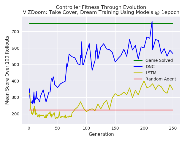
In the case of ViZDoom: Take Cover, a predictive model was trained in the environment using MDN-LSTM and MDN-DNC. Each was trained for 1 epoch, on random rollouts of 10,000 games which recorded the frames from the game (pixels) and actions taken at each timestep. The model was then used to train a CMA-ES controller. Note that the controllers were trained in the “dream” environment simulated by the model, as done in World Models.
A simulation of the environment — “dream” — where the controller is used to train using the learned model only, rather than the actual environment.
The controllers were tested in the environment throughout the generations for a 100 rollouts at each test. The results are plotted below. The MDN-DNC based controller clearly outperformed the MDN-LSTM based controller, and solved the game (achieving a mean score of 750 over 100 rollouts).
Comparison of a DNC based model versus a LSTM based model, used for training a controller in ViZDoom: Take Cover. The DNC based controller outperforms the LSTM controller.
Pommerman
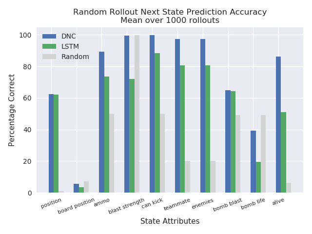
In the case of Pommerman, only the model’s predictions were used to test the capacity of the predictive model learned in a MDN-DNC and a MDN-LSTM. A controller was not trained. This was possible given that the states in Pommerman are coded as integers, rather than pixels. Thus, given [latex][s_t + a_t][/latex], the predicted state [latex][s_{t+1}][/latex] could be compared with the ground truth state from the actual game for equality, and to measure how many components of the state (position, ammo available, etc) were correctly predicted.
Here again, the MDN-DNC model outperformed the MDN-LSTM model, where both were trained exactly the same way for the same number of epochs. The MDN-DNC was more accurately able to predict the individual components of the next state given a current state and an action.
The predictive power of a DNC based model versus a LSTM based model in the Pommerman environment. The DNC based model was able to predict future states more accurately.
Conclusions
Model-based Reinforcement Learning or Evolution Strategies involve using a model of the environment when training a Reinforcement Learning or Evolution Strategies agent. In my case, the World Models approach to learn a predictive, probabilistic model of the environment in an Mixture Density Network was used. The Mixture Density Network consisted of a Differentiable Neural Computer, which output the parameters of a Gaussian mixture model that were used to sample the next state in a game. My experiments found that a model learned in a Differentiable Neural Computer outperformed a vanilla LSTM based model, on two gaming environments.
Future work should include games with long term memory dependencies, whereas with the experiments performed for this work it is hard to justify there being such dependencies in the ViZDoom: Take Cover and Pommerman environments. Other such environments would perhaps magnify the capabilities of the Differentiable Neural Computer. Also, what exactly is going on in the memory of the Differentiable Neural Computer at each timestep? It would be useful to know what it has learned, and perhaps features from the external memory of the Differentiable Neural Computer itself could be used when training a controller. For example, the Differentiable Neural Computer emits read heads, [latex]r_t[/latex], at each timestep, which are selected from the full memory, and used to produce the output (a prediction of the next state). Perhaps the contents of the read heads, or other portions of the external memory, could provide useful information of the environment if exposed directly to the controller along with the hidden state and cell state of the underlying LSTM.
World Models is a framework described by David Ha and Jürgen Schmidhuber: https://arxiv.org/abs/1803.10122. The framework aims to train an AI agent that can perform well in virtual gaming environments. World Models consists of three main components: Vision (V), Model (M), and Controller (C).
World Models Schematic
As part of my MSc Artificial Intelligence dissertation at the University of Edinburgh, I implemented World Models from the ground up in Chainer. My implementation was picked up by Chainer and tweeted:
According to OpenAI, Evolution Strategies are a scalable alternative to Reinforcement Learning. Where Reinforcement Learning is a guess and check on the actions, Evolution Strategies are a guess and check on the model parameters themselves. A “population” of “mutations” to seed parameters is created, and all mutated parameters are checked for fitness, and the seed adjusted towards the mean of the fittest mutations. CMA-ES is a particular evolution strategy where the covariance matrix is adapted, to cast a wider net for the mutations, in an attempt to search for the solution.
To demonstrate, here is a toy problem. Consider a shifted Schaffer function with a global minimum (solution) at f(x=10,y=10):
The fitness function F() for CMA-ES can be treated as the negative square error between the solution being tested, and the actual solution, against the Schaffer function:
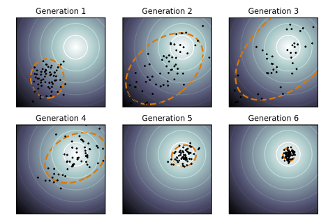
Therefore, the task for CMA-ES is to find the solution [latex](s_1=10, s_2=10)[/latex]. Given the right population size [latex]\lambda[/latex] and the right [latex]\mu[/latex] for CMA-ES, it eventually converges to a solution. With [latex]\lambda=64[/latex] and [latex]\mu=0.25[/latex], a visualization of CMA-ES as it evolves a population over generations can be seen below.
The animation below depicts how CMA-ES creates populations of parameters that are tested against the fitness function. The blue dot represents the solution. The red dots the entire population being tested. And the green dot the mean of the population as it evolves, which eventually fits the solution. You see the “net” the algorithm casts (the covariance matrix) from which the population is sampled, is adapted as it is further or closer to the solution based on the fitness score.
CMA-ES in action, quickly finding a solution to a shifted Schaffer function.