Context-Aware Prediction With Uncertainty of Traffic Behaviors Using Mixture Density Networks

Introduction

In autonomous driving, prediction is a measure of the future behavior of “agents” on the road. This typically includes behaviors (such as “lane following”, “turning left”, “turning right”), coupled with predicted trajectories consisting of (x, y) coordiantes. These predictions are then used by the Autonomous Vehicle’s (AV’s) planning and decision making modules, to ensure safe and optimal maneuvers that avoid collisions — for example, if a vehicle is predicted to come into the AV’s lane, the AV should respond accordingly by slowing down and allowing them to enter. The prediction problem can be complex, as scenes on the road can evolve very uniquely depending on the context such as number of agents on the road, road features, weather conditions, and so on. Additionally, the AV’s own behaviors affect the agents around it that predictions are sought for.

There is a plenty of literature proposing solutions to the traffic prediction problem using neural networks ([1], [2], [3] and many others) or probabilistic graphical models ([4], [5] and many others). However, I have not come across any work on solving it using Mixture Density Networks.

Mixture Density Networks (MDNs) [6], which I covered in a previous blog post, are neural networks that output the parameters of a mixture model, such as a Gaussian Mixture Model. MDNs are useful for tasks where a given input can potentially produce multiple outputs according to some probability. My post on MDNs shows the iconic toy problem where given an x coordinate, there could be multiple y coordinates. For example, given x=0.25, y could be {0, 0.5, 1} with perhaps equal probability of 1/3, 1/3, 1/3 per y coordinate. If such a problem is solved with neural networks trained with Mean Squared Error to produce a singular y output, it will likely only lead to the average y values — in the example aforementioned, y=0.5 for x=0.25.

Toy dataset of (x, y) coordiantes where certain x values map to multiple y values. The first image shows a 2D graph of the dataset’s ground truths. The second image shows the predictions of output y (in red) given input x, of a neural network trained on the dataset using Mean Squared Error. The third image shows the outputs (red) of a Mixture Density Network trained on the same dataset. The Mixture Density Network is adequately able to learn the distribution of the data.

The above example extends to traffic prediction very naturally. Let’s set up an example scene to explain why. An agent (a vehicle we are predicting for) approaches a Y-split in the road, and can go either right, or left. Depending on the agent’s past trajectory, perhaps one of the two options has a higher probability, though either is still probable up to a certain point. In this case, say we train a neural network regressor at this specific Y-split on past data of cars flowing through, using Mean Squared Error, to output a singular trajectory.

We can frame the inputs at timestep t as a series of (x, y) coordinates representing the past trajectory of the agent up to some P timesteps in the past, thus [latex]X_t = \{ (x_{t-P}, y_{t-P}), (x_{t-P+1}, y_{t-P+1}), …, (x_t, y_t) \}[/latex]. And the ouputs, the prediction, can be the agent’s trajectory up to some time horizon H in the future again consisting of coordinates at each timestep, thus [latex]Y_t = \{ (x_{t+1}, y_{t+1}), (x_{t+2}, y_{t+2}), …, (x_{t+H}, y_{t+H}) \}[/latex].

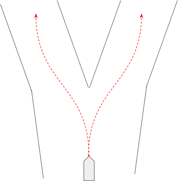
Take the scenario of traffic at a Y-split where agents can either go right or left with a 50/50 probability (up to a certain point before the Y-split) given a similar past trajectory. And say we have a balanced dataset of examples of these. Again, as seen in the toy example above, the Neural Network regressor trained with Mean Squared Error or the like, will end up giving an average of the two possible future trajectories, as depicted below. The image on the left shows the typical trajectories agents can take at this scene, and the image on the right shows the likely output trajectory of a vanilla neural network regressor trained on this scene.

As seen above, traffic scene prediction is a good candidate for where Mixture Density Networks can be used. In traffic scene prediction, we need a distribution over behaviors an agent can exhibit — for example, an agent could turn left, turn right, or go straight. Thus, Mixture Density Networks can be used to represent “behaviors” in each of the mixture it learns, where the behavior consists of a probability and trajectory ((x, y) coordinates up to some time horizon in the future). In the autonomous driving domain, it is helpful to have not just the predictions (the trajectories of agents around an autonomous vehicle), but the uncertainty attached to predictions, for better planning and decision making. A Mixture Density Network is a good candidate here additionally, as it will output a mixture of behaviors that have a probability (certainty) attached to each along with a standard deviation over the trajectories.

Problem Definition

In autonomous driving, data is typically gathered by the perception module, which consists of reading and logging sensors such as through video cameras, LiDaR, Radar, and so on. These sensors are meant to perceive the world and the state around the Autonomous Vehicle (AV), which include perceiving other agents on the road (vehicles, pedestrians, etc). In prediction (and other modules in the AV), raw sensor data such as images or point clouds can be used as input. Though I’ve read prediction papers where this raw data is used as input, a landmark paper by Waymo points to a number of papers that “show the brittleness of using raw sensor data” for learning to drive by means of prediction and planning [1] . Thus, some alternate pre-processing of raw sensor data is necessary. This data can be used to feed through neural network based object detectors, and a tracking module that uses perhaps the likes of Kalman filters to create traces of other agents on the road — individual agents tracked over time, using numeric representations of their dimensions (the size of the agent in meters, for example), position as a (x, y) coordinate, heading, velocity, and so on. Additionally, an HD map of the current location which includes features of the environment such as lanes represented as a series of (x, y) coordinates, can be used to place the perceived agents in the scene around the AV.

Example of an intermediate rasterized representation of a particular traffic scene at a particular timestep [2].

Where work on traffic prediction by Waymo [1], Uber [2], and others [3], create an intermediate rasterized (image) representation using this pre-processed data to feed to a convolutional network, I propose keeping it simple and feeding these numbers directly into a neural network without an intermediate representation expressed as an image. Thus, the input, [latex]X[/latex] can consists of a series of vectors representing the past positions (past trajectory) up to the current timestep, heading at the current timestep, and velocity at the current timestep, of individual agents in the scene. These inputs can be mapped to outputs, [latex]Y[/latex] — predictions of where the agents will be in some future time horizon such in the next 2 to 8 seconds from the present moment (their future trajectory).

Context is paramount in traffic prediction. For example, you observe a cyclist in a dedicated bike lane on a road going straight. And you also observe a vehicle stopped in the bike lane some distance ahead of the cyclist. Without taking the stopped vehicle into account, you would likely not be able to predict that the cyclist will have to pass the stopped vehicle by leaving the bike lane and coming into the vehicle traffic lanes. Thus, context must include other agents that may or may not affect a particular agent we are predicting for. Features of the current scene also provide important context, that must be taken into account. For example, the contours of the lane (if they curve right, an agent following the lane will need to adjust accordingly), locations and states of traffic lights (traffic light is red, so agents will likely stop as they approach), traffic rules (one way roads, etc), and so on.

For the traffic prediction problem, I propose a single feedforward neural network that at a given timestep [latex]t[/latex] can take up to some [latex]N[/latex] agents as inputs (their past trajectories up to some [latex]t-P[/latex] timesteps) and produce [latex]N-1[/latex] outputs for predictions of their future trajectories up to some time horizon [latex]t+H[/latex]. The [latex]N[/latex] agents include the ego vehicle (the AV), as the position and movement of the ego vehicle itself may affect other agents around it and can provide context for predictions for the others, and then [latex]N-1[/latex] of the closest agents to the ego based on euclidean distance, as predictions for irrelevant agents such as those much further away than the AV are not necessary. This consolidated input will provide multi-agent context to the network, allowing it to learn interactions among agents and how that relates to predictions of their future trajectories. The outputs need only include the trajectories of the [latex]N-1[/latex] closest agents, as we need not predict for the AV.

More specifically, at a given timestep [latex]t[/latex], the input for each agent, [latex]X[/latex], can include their past trajectory of (x, y) coordinates up to some [latex]P[/latex] previous timesteps, their heading, their velocity, and additionally I propose the lane contours of the lane they are currently in expressed as (x, y) coordinates. Thus, for each agent [latex]n[/latex], [latex]X^n_t = \{ (x_{t-P}, y_{t-P}), (x_{t-P+1}, y_{t-P+1}), …, (x_t, y_t), heading_t, veolcity_t, (x^{lane}_1, y^{lane}_1), (x^{lane}_2, y^{lane}_2), …, (x^{lane}_?, y^{lane}_?) \}[/latex]. The outputs for each agent [latex]n[/latex] includes their trajectory up to some future time horizon [latex]H[/latex], thus [latex]Y^n_t = \{ (x_{t+1}, y_{t+1}), (x_{t+2}, y_{t+2}), …, (x_{t+H}, y_{t+H}) \}[/latex]. Following these, the full input to the neural network at a single timestep would be the ego-centric (from the perspective of the AV) “scene” [latex]I_{t} = \{ X^1_t, X^2_t, …, X^N_t \}[/latex] and full output would be [latex]O_{t} = \{ Y^1_t, Y^2_t, …, Y^{N-1}_t \}[/latex]. Note that in order to make this a feasible and somewhat consistent (“normalized”) problem for the neural network to learn, all euclidean (x, y) coordinates can be made relevant to the AV’s current position at the current timestep. That is, setting [latex](x^0_{t=0}, y^0_{t=0}) = (0.0, 0.0)[/latex], and having all other coordinates of all agents trajectory positions and lane contours offset relatively.

As a simple feedforward neural network (as opposed to a more complex LSTM setup) will be used, unfortunately the input and output sizes will need to be fixed. This is somewhat problematic because we have to know up front how many agents are in a given scene, and additionally, how many behaviors we want the MDN to predict (as in, number of mixtures — more on that below). For example, if the network is trained using input that includes the ego vehicle plus the 9 closest agents, but only 3 other agents are observed. However, this can be overcome as we can zero-pad all inputs and outputs if none are available at any given timestep. In the aforementioned example, all inputs and outputs for the additional agents can just consist of all 0’s.

Mixture Density Network Setup

As a MDN is being used for this problem, the neural network does not output [latex]O_{t}[/latex] directly. Instead, it outputs a set of mixture coefficients (probabilities attached to each mixture) [latex]\alpha[/latex], means [latex]\mu[/latex], and standard deviations [latex]\sigma[/latex] — the parameters of a Gaussian Mixture Model (GMM). These parameters can then be sampled from to get [latex]O_{t}[/latex] for predicted future trajectories for the individual agents, which are used along with the uncertainty of each trajectory expressed as a probability and standard deviation of the trajectory, to feed into the AV’s planning module.

While the MDN can be framed to output a Gaussian mixture, [latex]\{\alpha^{1:K}_t, \mu^{1:K}_t, \sigma^{1:K}_t \}[/latex] where [latex]K[/latex] is the number of desired mixtures, for each individual (x, y) euclidean coordinate in the trajectory, it can instead be biased to learn behaviors in the mixtures. Instead of making every point a mixture, we can move the mixture to a higher level where the mixture represents a set of (x, y) coordinates — the trajectory — as a whole, and thus, map to a certain behavior. In this setup, each “behavior” is intended to represent a high-level behavior an agent on the road could exhibit, such as “go left”, “go right”, “go straight”, and so on.

We can represent behaviors as [latex]B^{1:K}_t[/latex], where [latex]K[/latex] is the number of mixtures output for the GMM being represented by the MDN. Each behavior [latex]B^k_t[/latex] can have a coefficient [latex]\alpha^{k}_{t}[/latex] representing the probability of the likelihood of that mixture, so [latex]\sum_{k=1}^{K} \alpha^k_t = 1[/latex]. Additionally, each behavior contains a set of (x, y) coordinates up to a time horizon [latex]H[/latex] represented as means [latex]M^k_t = (\mu^{x, k}_{t+1:t+H}, \mu^{y, k}_{t+1:t+H})[/latex], to produce the predicted trajectory defined earlier: [latex]Y_t = \{ (x_{t+1}, y_{t+1}), (x_{t+1}, y_{t+1}), …, (x_{t+H}, y_{t+H}) \}[/latex]. For the standard deviation [latex]\sigma[/latex], it can be taken per (x, y) coordinate as a whole, rather than individually for each x and each y. The standard deviation then represents the uncertainty of the coordinate as a whole — so per behavior [latex]k[/latex], in [latex]K[/latex] total behaviors, we have [latex]S^k_t = \sigma^{k}_{t+1:t+H}[/latex].

The predicted behaviors per agent per timestep [latex]t[/latex] can be represented as [latex]B^k_t = \{\alpha^k_t, M^k_t, S^k_t\}[/latex]. If for our MDN we have [latex]N[/latex] agents as input — the ego vehicle (the AV) and [latex]N-1[/latex] closest agents in euclidean distance — the desired outputs include predicted behavior of the N-1 closest agents. The full output [latex]O_t[/latex] of the neural network in the MDN is then [latex]\{ B^{1, 1:K}_t, B^{2, 1:K}_t, …, B^{N-1, 1:K}_t \}[/latex].
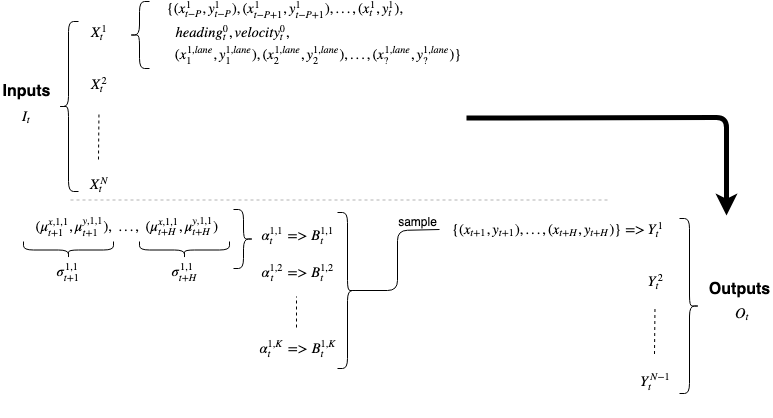
Inputs and Outputs of Mixture Density Network for traffic behavior prediction. Zero-filled where data is not available.

The number of mixtures (the number of behaviors) is an open question, and will likely require some thought and experimentation. However, a good starting point would be 3, simply based on the intuition that in traffic, a vehicle can go left, right, or straight. Left or right could mean switch lanes or a full left or right turn, which the network should learn based on the usual behavior and lane contours in the scene.

[2]’s approach to traffic prediction involves using a neural network outputting a single behavior for an agent as a trajectory of (x, y) coordinates up to some future time horizon. Additionally, they output a standard deviation per each (x, y) coordinate in the trajectory. [2] find empirically that training such a network requires curriculum, where the network is first trained with the Mean Displacement Error, and then the standard deviation outputs are trained. Note that the Mean Displacement Error simply involves taking the mean of the euclidean distance of each point in the predicted trajectory with the ground truth trajectory. The equations for calculating the Mean Displacement Error, and the half-Gaussian loss including the standard deviation can be seen in the figure below.
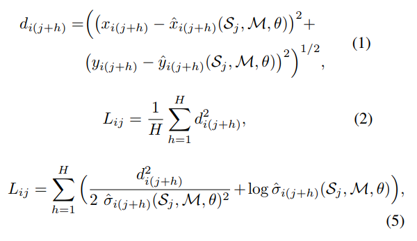
[2]’s loss functions. Equation 1 represents the displacement error between the predicted and ground truth (x, y) coordinates. Equation 2 represents the Mean Displacement Error which the network is first trained with. Equation 5 represents the full half-Gaussian loss function which includes the displacement error.

The MDN can be trained similarly via curriculum where first the network is trained with Mean Displacement Error, where the means ([latex]mu[/latex]’s) of the (x, y) coordinates output for each mixture for each agent are trained, and then the full outputs including the standard deviation’s ([latex]\sigma[/latex]’s) are trained using the half-Gaussian distribution loss. The main difference is that we need to train additionally for multiple outputs (behaviors/mixtures) per individual agent, and thus also train the MDN coefficients [latex]\alpha[/latex]’s. This can simply be done by taking a softmax of the coefficients and multiplying them with the mean loss for each mixture, and then taking the sum of the loss across all mixtures. That is, [latex]L_{total} = \sum_{k=1}^{K} \alpha^k L_{ij}[/latex] where [latex]L_{ij}[/latex] are the losses either from equation (2) or (5) displayed from [1]’s approach, depending on which part of the curriculum is being trained.

Additionally, as this is a complex problem for the network to learn, I propose applying another curriculum to the training by progressively training for the number of agents in the output starting from number of trainable agents = 1. Meaning, first train the mixtures output for the first agent (agent 1) only, by a) using Mean Displacement Error first and b) full half-Gaussian second, and then training the first two agents together (agents 1 and 2) similarly, and so on up to all agents in the full output.

Code for this loss function in Python, using Chainer, is displayed below. The input variable holds the full input at some timestep as mentioned earlier (past trajectories and lane contours of an ego vehicle and its closest [latex]N-1[/latex] agents). The num_agents represents the total number of agents in the inputs and outputs. trainable_agents represents the number of agents in the curriculum being currently trained for as described earlier (1, 1:2, 1:3, 1:4, …, 1:N-1). And finally output holds the ground truth trajectory of (x, y) coordinates for each agent being predicted for, up to future some time horizon.

coef, mu, ln_var = self.fprop(input)

coef = coef.reshape(output.shape[0], num_agents, num_mixtures)
coef = F.softmax(coef, axis=2)
mu = F.reshape(mu, (output.shape[0], num_agents, num_mixtures, -1, 2))
ln_var = F.reshape(ln_var, (output.shape[0], num_agents, num_mixtures, -1))

output = output.reshape(output.shape[0], num_agents, 1, -1, 2)
output = F.repeat(output, num_mixtures, 2)

coef = coef[:, :trainable_agents, :]
ln_var = ln_var[:, :trainable_agents, :, :]

x_true = output[:, :trainable_agents, :, :, 0]
y_true = output[:, :trainable_agents, :, :, 1]
x_pred = mu[:, :trainable_agents, :, :, 0]
y_pred = mu[:, :trainable_agents, :, :, 1]

if curriculum_step == 1:
    loss = F.sum(coef * F.sum(((x_true-x_pred)**2) + ((y_true-y_pred)**2), axis=3))
else:
    displacement_sq = ((x_true-x_pred)**2) + ((y_true-y_pred)**2)
    ln_var = F.clip(ln_var, -300., 300.) #Numerical stability
    var = F.exp(ln_var)
    loss = F.sum(coef * F.sum(((displacement_sq/(2*var)) + F.log(F.sqrt(2 * math.pi * var))), axis=3))

Data

The data can originate from either sensors on an AV driving around, or fixed CCTV style cameras pointed at a road. In either case, it will be necessary to track agents in the scene at a given moment with an identifier, and preprocess the sensor or video footage into “traces” — a vector of (x, y) coordinates observed for the agent’s position over time, expressed in a particular reference system, as the agents enter and exit the vicinity of the AV or fixed camera.

These traces can then be divided into inputs and outputs to form a dataset in the following manner. As an example setup, if an agent is seen for a total of 15 seconds at a frame rate of 25 Hz, that gives us 375 total observed positions of the agent over time. If we set the prediction time horizon (referenced as [latex]H[/latex] previously) to 2 seconds at 25 Hz (thus 50 future positions desired for prediction), based on an input of the past 1 second of the agent’s past positions (25 past positions), our inputs and outputs can be divided from the total 375 frames available for the agent, for every timestep [latex]t \in \{0:325\}[/latex]. At each timestep [latex]t[/latex], the dataset for this agent can contain input = [latex]\{(x_{t-25}, y_{t-25}), …, (x_t, y_t)\}[/latex] and output = [latex]\{(x_{t+1}, y_{t+1}), …, (x_{t+50}, y_{t+50})\}[/latex]. At timestep [latex]t = 0[/latex], as positions are not available from the previous 1 second for the agent, the input can be zero-filled.

Additionally, for adding in the environmental context, an HD map of the locations the agent traces are collected from will be required. This map can provide the lane contours for each agent for the inputs.

All data for inputs, outputs, and lane contours, should be ego-centered. Meaning, for the ego vehicle in the input, the current (x, y) position at [latex]t=0[/latex] would be (0.0, 0.0), and all other (x, y) positions should be relative to this, to normalize the data for the neural network.

Results

Experiments were performed on a proprietary dataset consisting of 24 hours of detection at a fixed scene, using the following setup and hyperparameters:

ParameterSetting
Number of mixtures3
Past positions of agents, P1 second = 25
Time horizon for prediction, H2 seconds = 50
Ego vehicle + number of closest agents1+9 = 10
Distance to find closest agents40 meters
Number of layers10
Hidden units1024
ActivationsReLU

The dataset was split into train, validation and test sets. After curriculum training the MDN as described above to a point where satisfactory results were achieved on the validation set, predictions on the test set were compared against the ground truths using Root Mean Squared Error (RMSE), using the Manhattan distance between the coordiantes. This RMSE was compared to an implementation of DESIRE [3], which was trained and tested on the same dataset.

While DESIRE achieved an RMSE of 0.38979 on the test set, the MDN achieved an RMSE of 0.401587, when testing only the first agent’s output. When testing all 9 agent’s outputs against the ground truths, the MDN achieved an RMSE of 0.478878 (when using the trajectory from the most likely behavior). Note that with DESIRE, only a single agent’s prediction is tested at a time. Furthermore, DESIRE constitutes a series of complex LSTMs with several expensive intermediate steps, whereas the MDN can achieve similar results for multiple agents at a time, in a single forward pass with a simpler feedforward network.

Upon inspecting the results in detail, I also noticed that the mixtures were appropriately mapping to plausible high-level behaviors with adequate probabilities given the agent’s history, particularly in situations where there was ambiguity in where the agent could go next. I also observed in many cases the probability being almost 1 ([latex]\alpha=1[/latex]) for a behavior for agents where the network strongly expressed they could only go in a certain direction given their past trajectory. Otherwise, the performance and learning of the behaviors will require more quantitative experiments to measure, as the definition and ground truths of behavior are harder to measure as opposed to raw predicted trajectories being compared using RMSE.

Conclusions

For the traffic prediction problem, Mixture Density Networks (MDN) can be used to learn a distribution over agents’ trajectories in a traffic scene. If the MDN is framed to produce a full trajectory within each Gaussian mixture as a whole, as opposed to framing each point in the trajectory to be a mixture in its own, the MDN can be biased to learn higher-level behaviors of agents, leading to more accurate and plausible predictions. These behaviors come with a probabilities at the behavior level, and standard deviation over the trajectory predictions, allowing for uncertainty-aware decision making in the Autonomous Vehicle context.

This method can achieve similar prediction accuracy to state-of-the-art methods such as DESIRE [3], when measuring the Root Mean Squared Error of the Manhattan distance of the predicted coordinates in the trajectories to the ground truths. While state-of-the art methods may require series of complex neural networks such as LSTMs, with expensive intermediate processing steps, the MDN can achieve similar results for multiple agents at a time, in a single forward pass with a simple feedforward network, using no intermediate rasterized representation.

The limitations with this approach are that the number of agents being input and output, and the number of mixtures and thus behaviors, are fixed at train time. To overcome this limitation, perhaps in future work RNNs can be explored for feeding inputs and receiving outputs as sequences that are terminated with separator markers, similar to how the dataset is composed to train and test the Differentiable Neural Computer:
https://github.com/AdeelMufti/DifferentiableNeuralComputer. Furthermore, in future work, this method should be trained and tested on a variety of scenes, with an ablation study to determine how much the multi-agent and environmental context helps with prediction. The number of Gaussian mixtures also requires further consideration and experimentation.

References

[1] Mayank Bansal et al., ChauffeurNet: Learning to Drive
by Imitating the Best and Synthesizing the Worst
, 2018, https://arxiv.org/abs/1812.03079.
[2] Nemanja Djuric et al., Short-term Motion Prediction of Traffic Actors for Autonomous Driving using Deep Convolutional Networks, 2018, https://arxiv.org/abs/1808.05819.
[3] Namhoon Lee et al., DESIRE: Distant Future Prediction in Dynamic Scenes with Interacting Agents, 2017, http://www.robots.ox.ac.uk/~tvg/publications/2017/CVPR17_DESIRE.pdf.
[4] Jens Schulz et al., Interaction-Aware Probabilistic Behavior Prediction in Urban Environments, 2018, https://arxiv.org/abs/1804.10467.
[5] Jingbo Zhou et al., R2-D2: a System to Support Probabilistic Path Prediction in Dynamic Environments via “Semi-Lazy” Learning, 2013, https://www.researchgate.net/publication/262271558_R2d2_A_System_to_Support_Probabilistic_Path_Prediction_in_Dynamic_Environments_via_semilazy_Learning.
[6] Christopher M. Bishop, Mixture Density Networks, 1994, https://publications.aston.ac.uk/373/1/NCRG_94_004.pdf.

Reinforcement Learning using Intrinsic Rewards through Random Network Distillation in Chainer

➡ Implementation: https://github.com/AdeelMufti/RL-RND

Intrinsic Motivation is all the rage in Reinforcement Learning these days. In human psychology, intrinsic motivation refers to behavior that is driven by internal rewards. One example of intrinsic motivation is, if something new and usual is encountered, it may cause someone to give it more attention. In RL, a fine balance between exploration and exploitation is required. If exploration is inadequate, an agent may get stuck in a local optimum. This is particularly problematic if extrinsic rewards are sparse or not well defined. Thus, a mechanism for intrinsic motivation can be used to cause the agent to explore.

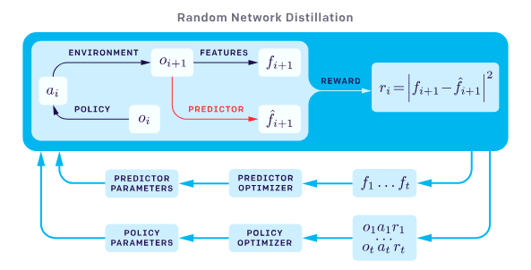
Enter Random Network Distillation (RND), as proposed by OpenAI:
https://openai.com/blog/reinforcement-learning-with-prediction-based-rewards/. In summary, a randomly initialized network — the target — is used to distill another network — the predictor — by training the predictor to learn the output of the target network given all states encountered so far as input. The measure of error between the target network and predictor network, can be used as a metric for intrinsic motivation when training a RL agent. As the target network and predictor network process states they repeatedly see while the RL agent does rollouts in the environment, the predictor network learns the target network’s reaction to the states, and thus the intrinsic reward becomes increasingly lower as the same state is seen again and again. However, if a new state is encountered, the predictor network would not be aligned with the target network on the new state, thus producing a spike in the error and increase in intrinsic motivation, allowing the agent to explore the new state encountered due to the higher rewards.

I decided to create my own implementation in Chainer of a Proximal Policy Optimization (PPO) RL agent, to use intrinsic rewards through Random Network Distillation. I kept the implementation as close as possible to the details in OpenAI’s paper. The implementation can be seen at:
https://github.com/AdeelMufti/RL-RND.

I conducted an experiment with PixelCopter-v0, which I’ve been dealing with as a baseline task for a series of experiments involving Reinforcement Learning, Evolution Strategies, and Differentiable Neural Computers. I’ve noted that for several learning algorithms (CMA-ES, PPO, Policy Gradients), the agent easily and quickly falls into a local optimum. It goes up a few times (action = up), and then after that all actions are “no action”, until it falls on the floor and the game is over. This allows it to get a higher score than with random actions, but after that it never improves. When experimenting with PPO with RND for intrinsic motivation, I turned off the external rewards. Very interestingly, the agent fell into that exact local optimum, simply based on the intrinsic rewards!

As I conduct more experiments and adjust my implementation, I will be updating this post.

Differentiable Neural Computer Memory Testing Using dSprites

Introduction

These negative results can hopefully provide important information for others working with the Differentiable Neural Computer (DNC). In this post I’ll cover a series of experiments I performed to test what is going on in the external memory of a DNC, without being able to find anything positively conclusive. This was a followup exercise to my work on Probabilistic Model-Based Reinforcement Learning Using The Differentiable Neural Computer.

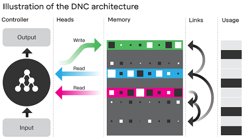
The DNC is a form of a memory augmented Neural Network that has shown promise on solving complex tasks that are difficult for traditional Neural Networks. When a Recurrent Neural Network (RNN) such as Long Short Term Memory (LSTM) is used in the DNC architecture, it has the capacity to solve and generalize well on tasks with long temporal dependencies across a sequences. At each timestep in a sequence, the DNC receives an external input, and memory data read from its internal read head mechanism from the previous timestep, to manipulate its internal state and produce the next output.

The external memory of the DNC also presents an additional mechanism to observe what the DNC is doing at each timestep. DeepMind did some evaluation of the memory contents in their original paper on Neural Turing Machines on some very structured problems it was trained on (such as copying), to infer it was learning algorithms as the memory contents recorded and moved information in structured ways.

In my previous work, I used DNCs for model-based Reinforcement Learning, where a model of video games was learned in the DNC. Features from this model were then used to train a controller to maximize its cumulative rewards in the video game. The features fed to the controller from the model were the hidden state [latex]h_t[/latex] and cell state [latex]c_t[/latex], of the LSTM in the model, at every timestep [latex]t[/latex], as done in the World Models framework.

I conjectured that the memory of the DNC used to train a model of the environment could contain useful information that could augment the the hidden and cell states of the LSTM being fed to a controller. At each timestep, the DNC contains the contents of its full memory ([latex]M_t[/latex]), portions of which are read by the read heads ([latex]r_t[/latex]) and used to produce the next output. Perhaps [latex]M_t[/latex] or [latex]r_t[/latex] contain useful information for the controller, especially if the video game contains very long term dependencies that need to be tracked as the game progresses.

Experiment Setup

I decided to test what information is contained in the DNC’s memory at each timestep, when a predictive model of the environment is trained using a DNC as in the World Models framework. A “Model” in World Models is trained using Teacher Forcing, where the state of the game, z, at each timestep, along with an action, a, to be performed at that state, is given as input to the model. The model uses this information to predicts the next state. The state in this case is a compressed, “latent”, representation of the frame (image expressed as pixels) from the game at each timestep, created using a Convolutional Variational Autoencoder (CVAE). More specifically, the model receives input [latex][z_t + a_t][/latex] and produces output [latex]z_{t+1}[/latex].

As I found with my work on Probabilistic Model-Based Reinforcement Learning Using The Differentiable Neural Computer, DNC based models trained this way were able to outperform their vanilla LSTM (without external memory agumentation) counterparts. But, what is going on in the DNC’s external memory when it is trained this way? And furthermore, can this information be useful to a Reinforcement Learning or Evolution Strategies controller?

One way to test would be to check if the memory contained, linearly separable information about the current state. But to do so would require some discrete state labels of the video game for which a model was being learned, that could be used as ground truths. These states are not easily available or obvious when a model of the game is being learned from frames (images expressed as pixels) from live gameplay. Thus, with the help of a colleague, I formulated a toy task using DeepMind’s dSprites dataset.

dSprites consists of 737,280 total images that come from combinations of 5 different classes:

  1. Shape: square, ellipse, heart
  2. Scale: 6 values linearly spaced in [0.5, 1]
  3. Orientation: 40 values in [0, 2 pi]
  4. Position X: 32 values in [0, 1]
  5. Position Y: 32 values in [0, 1]
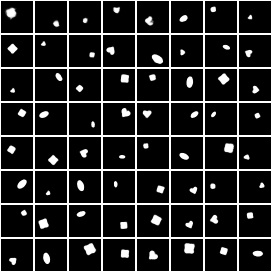
Examples of randomly selected “sprites” from the dSprites dataset.

To train a predictive model using dSprites, I created rollouts to mimic what a video game would do. A rollout starts with a randomly selected sprite, and the “action” at each timestep provides information about the next sprite, also randomly selected (since this is not a real game). The actions correspond to the classes of the sprites, but more specifically, are the difference between the classes of the sprites from previous timesteps. If the classes of the sprites are represented at each timestep [latex]t[/latex] as [latex]\hat{a}_t[/latex], and the actual action provided to the model is represented as [latex]a_t[/latex], then [latex]a_t = \hat{a}_{t} – \hat{a}_{t-1}[/latex], where [latex]a_0 = 0[/latex]. As with the World Models teacher forcing training to learn a predictive model of the game, the state (the image of the current sprite) and action (classes delta to achieve the next sprite) are concatenated and input together to the model to predict (as output) the image of the next sprite. This setup allows the model to couple the state (the image of the sprite) with the action together to learn what the next sprite should be, rather than depending solely on the action if the action directly provided the classes of the next sprite, as that signal would be too strong and potentially cause the network to ignore the state input altogether.

As an example of the action inputs at each timestep, take our first randomly selected sprite to be [latex]\hat{a}_0[/latex] = [shape=1, scale=0.6, orientation=3.14, position_x=0.0625, position_y=0.0625]. The first input provided to the model would be the image of this sprite concatenated with action [latex]a_0[/latex] = [shape=0, scale=0, orientation=0, position_x=0, position_y=0] (by definition). Then, if the classes for the next randomly selected sprite are [latex]\hat{a}_1[/latex] = [shape=1, scale=0.7, orientation=0, position_x=0.125, position_y=0.125], the next action would be [latex]a_1 = \hat{a}_1 – \hat{a}_0[/latex] = [shape=0, scale=0.1, orientation=-3.14, position_x=0.0625, position_y=0.0625]. And so on.

Using this setup, rollouts of random length between 500 to 1000 were used to train the model, for 10,000 rollouts per epoch, for 5 epochs. Note that no CVAE or Mixture Density Network was used as is done in the World Models framework. This was to allow the model to be entirely deterministic, to make testing of memory more consistent.

Two variants of the DNC were trained, Model A and Model B:

Model A
Memory lengthN = 256
Memory widthW = 64
Number of read headsR = 4
Total memory size16384
Read heads size256
Model B
Memory lengthN = 16
Memory widthW = 16
Number of read headsR = 4
Total memory size256
Read heads size64

After training the DNC models, tests on the content of the memory were performed as follow. For each test, the model was run through 10,000 rollouts as described above, for a fixed sequence of length 500, and the contents of the full memory [latex]M_t[/latex] (in the case of Model B only) and contents of the read heads [latex]r_t[/latex] (both models), were logged at each timestep. Additionally, the full class label ground truths of the randomly selected sprites were logged at each timestep.

Test 1

This test was designed to check whether the logged full memory or read heads of the models contained information that could be used to infer the classes of the sprite at each timestep. As mentioned earlier, at each timestep, provided to the model as input are the current “state” which is the image of the current sprite, and the “action” which is the delta of the current sprite’s class label from the next randomly selected sprite’s class label, to allow the model to learn to use the two combined to predict the next state (the image of the next randomly selected sprite).

The test included checking whether at the current timestep, the memory contents could be used to infer the class labels of the current sprite being input. And whether it could be used to infer the class labels of past sprites it had already seen — 5 timesteps ago and 10 timesteps ago. Thus, each test was to check if the memory contained information about the class labels of the sprites presented at timesteps a) t-0, b) t-5, and c) t-10.

To do so, a simple single layer feedfroward neural network, without any activations, was used to train to use the memory contents (either full memory or just the read heads) at each timestep as input, to predict the class labels of the sprites at past timesteps as output. The point of doing it this way was to check whether the information being sought (the class labels) was clearly present in the memory by being linearly separable. It is inspired by the [latex]\beta[/latex]-VAE paper.

The neural network was trained using Softmax Cross Entropy loss for the shape class, and the Mean Squared Error loss on the scale, orientation, X position, and Y position classes. It was trained for a single epoch on the 10,000 rollouts with the logged memory contents at each timestep of the rollout sequence as inputs and class labels at each timestep of the rollout sequence as outputs. The Adam optimizer was used, with a minibatch size of 256. The inputs (the memory contents) were normalized by subtracting the mean and dividing by the standard deviation at each timestep.

After training, as this was a simple linear separability test to determine if the class labels could be easily inferred from the data, the same train set was used to test and compare the predicted classes with the ground truth classes using classification error for the shape label, and Mean Squared Error for the scale, orientation, X position, and Y position labels.

Test 2

The second test was designed to check whether if a pattern of “actions” (sprite classes) were given to the model in a predetermined sequence of length T (no longer of random length), if this pattern could be seen in the DNC’s external memory when logged and analyzed, using Mutual Information. The test involved running the model through a sequence of X positions, and this sequence was then checked using the mutual information score against each memory location by iterating over all memory locations and using the contents at that specific location over the timesteps.

For example, Model B had a full memory size of 256, which meant that each location in memory from 0 to 255 had some content, for every timestep from 0 to T of the input sequence the model was provided. If the X positions were fixed to be [0, 15, 30, 15, 0] (T=5), then first, memory location 0’s contents over the 5 timesteps, [?, ?, ?, ?, ?], were checked against the fixed X position sequence using mutual information score. Then memory location 1’s contents over the timesteps. And so on.

The point of this test was to check if the DNC had learned class representations of dSprites and was using the memory to track discrete information about the sprite’s classes — in this case, the X position of the sprites.

Results

Both DNC models were able to learn to predict the next state, i.e. the image of the next sprite, fairly well, based on visual inspection. Below, the real sprites are to the left, and predicted sprites to the right, from Model A. Note that the models are trained to output the full image of the sprite directly.

Test 1

As a control, random inputs instead of the memory contents, were provided to the simple linear neural network model, but trained to predict the true labels. This linear model produced the following results:

Random Input Results:
shape classification error=0.6672701999999999
scale mse=0.030593501669909217
orientation mse=3.478348739661164
position_x mse=0.09114251257732676
position_y mse=0.0913002843063043

Model A’s memory contents used were the read heads [latex]r_t[/latex] of size 256, and the simple linear model produced the following results in predicting the ground truth labels:

Model A Read Heads Results:
shape classification error=0.5730384
scale mse=0.029882248834080166
orientation mse=3.454711805402036
position_x mse=0.02671479350697897
position_y mse=0.01284542320401027

Model B’s memory contents used were the full memory [latex]M_t[/latex] of size 256, and simple linear model produced the following results in predicting the ground truth labels:

Model B Full Memory Results:
shape classification error=0.6396944
scale mse=0.02892420274878035
orientation mse=3.3985103721710175
position_x mse=0.08951739388579043
position_y mse=0.08840673772025909

Additionally, Model A was tested using the simple linear model trained on Model A’s read head contents at each timestep but instead using class labels from t-5 time steps ago and t-10 timesteps ago, to check if the memory contained information about past classes. Similarly, Model B was tested using the simple linear model trained on Model B’s full memory contents at each timestep. In both cases, the results were significantly worse than those listed above (i.e. predicting class labels at timestep t-0), and were close to the results from the random inputs, hence have been omitted from this post for brevity.

Test 2

For the second type of test, rollouts with all classes fixed except for the X position, were used as input. 50 sequences were created that randomly shifted the X position class between its 32 possible values, for a random length (number of timesteps in each rollout). These sequences of class labels were used as actions as described earlier, and the corresponding sprite images, were together fed as input to both Model A and Model B, and the content of the full memory [latex]M_t[/latex] at each timestep was logged. The memory content at each location within the memory was then tested to contain this predetermined sequence using the mutual information score

Additionally, during each of the 50 tests, a random sequence of class label inputs was created that was of the same length as the ground truth test sequence. This random sequence also ranged randomly between the 32 possible X position class values. The memory content at each location was also tested against this entirely random sequence, as a control.

For all sequences tested, contents at each location in the full memory were compared with the true test sequence for X position and the random control sequence. The mutual information score was roughly the same for both sequences, and less than 1e-8, for every memory location, thus showing virtually no mutual information in the memory contents.

Conclusions

The purpose of these experiments was to check when training a DNC to learn a predictive model of an environment such as a video game, whether the DNC’s external memory contained information about the states in the environment. The dSprites dataset was used to create a toy environment, as the sprites have class labels that can be used to map to discrete states the environment is in.

Test 1 was designed to check whether the full memory contents together, or the read head contents together, contained linearly separable information about the sprite classes being input at each timestep. However, in all experiments performed, the contents of the memory provided only very marginally better information in predicting the classes than when using random inputs instead of the memory contents. Model A’s read head contents performed slightly better than the random inputs compared to Model B’s full memory contents, particularly on the position classes. This points to a conjecture that perhaps the read head contents when training a DNC predictive model with a larger memory matrix can provide some useful information about the state of an environment. However, strong results should have seen significant improvement (lower errors, closer to zero) over predicting the states when using the memory contents compared to random inputs.

Test 2 was designed to check whether the DNC had learned some representation of the classes of dSprites when training a predictive model, and was using individual locations in the memory to track information about the states (classes) of the sprites being input. The tests showed that the DNC was not tracking the class that was tested, the X position, in any deterministic location in its memory, when using a mutual information score. In all tests, the score was close to zero, and no better than a random control sequence additionally tested at each memory location.

In future work, experiments could be performed to check whether the memory contains information about each individual classes in isolation. Also, perhaps the predictive model of the environment can be trained in a different manner such as with an augmented loss function, to bias the DNC in exposing more information about the state in its memory. Lastly, the Pygame Learning Environment has games where a discrete encoded state representation of the game can be queried at each timestep, and perhaps the DNC’s memory can similarly be tested on these environments as this representation gives labels for the states.

Probabilistic Model-Based Reinforcement Learning Using The Differentiable Neural Computer

My experiments found that a model learned in a Differentiable Neural Computer outperformed a vanilla LSTM based model, on two gaming environments.

➡ Thesis PDF: http://adeel.io/MSc_AI_Thesis.pdf

Introduction

For my MSc Artificial Intelligence at the University of Edinburgh, my dissertation included 4 months of research. I investigated the use of the Differentiable Neural Computer (DNC) for model-based Reinforcement Learning / Evolution Strategies. A predictive, probabilistic model of the environment was learned in a DNC, and used to train a controller in video gaming environments to maximize rewards (score).

The difference between Reinforcement Learning (RL) and Evolution Strategies (ES) are detailed here. However, in this post and my dissertation, the two are used interchangeably as either is used to accomplish the same goal — given an environment (MDP or partially observable MDP), learn to maximize the cumulative rewards in the environment. The focus is rather on learning a model of the environment, which can be queried while training an ES or RL agent.

The authors of the DNC conducted some simple RL experiments using the DNC, given coded states. However, to the best of my knowledge, this is the first time the DNC was used in learning a model of the environment entirely from pixels, in order to train a complex RL or ES agent. The experiments I conducted showed the DNC outperforming Long Short Term Memory (LSTM) used similarly to learn a model of the environment.

Learning a Model

The model architecture is borrowed from the World Models framework (see my World Models implementation onGitHub). Given a state in an environment at timestep t, [latex]s_t[/latex], and an action [latex]a_t[/latex] performed at that state, the task of the model is to predict the next state [latex]s_{t+1}[/latex]. Thus the input to the model is [latex][s_t + a_t][/latex], which produces output (prediction) [latex]s_{t+1}[/latex]. Note that the states in this case consist of frames from the game at each timestep consisting of pixels. These states are compressed down to latent variables z using a Convolutional Variational Autoencoder (CVAE), therefore more specifically the model maps [latex][z_t + a_t] => z_{t+1}[/latex].

The model consists of a Recurrent Neural Network, such as LSTM, that outputs the parameters of a Mixture Density Model — in this cased, a mixture of Gaussians. This type of architecture is known as a Mixture Density Network (MDN), where a neural network is used to output the parameters of a Mixture Density Model. My blog post on MDNs goes into more details. When coupled with a Recurrent Neural Network (RNN), the architecture is known as MDN-RNN.

Thus, in learning a model of an environment, the output of the MDN-RNN “model” is not simply [latex]z_{t+1}[/latex], but the parameters of a Gaussian Mixture Model ([latex]\alpha, \mu, \sigma[/latex]) which are then used to sample the prediction of the next state [latex]z_{t+1}[/latex]. This allows the model to be more powerful by becoming probabilistic, and encode stochastic environments where the next state after a given state and action can be one of multiple.

For the experiments I conducted, the architecture of the model used a DNC where the RNN is used in World Models, thus, the model is composed of a MDN-DNC. Simply, the recurrent layers used in the MDN are replaced with a DNC (which itself contains recurrent layers that are additionally coupled with external memory).

The hypothesis was that using the DNC instead of vanilla RNNs such as LSTM, will allow for a more robust and algorithmic model of the environment to be learned, thus allowing the agent to perform better. This would particularly be true in complex environments with long term dependencies (meaning, a state perhaps hundreds or thousands of timesteps ago needs to be kept in context for another state down the line).

Experiments And Results

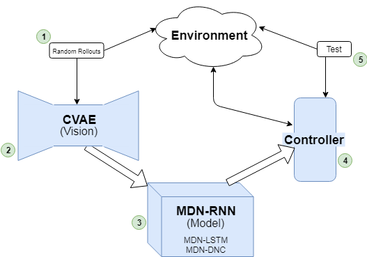
Experimentation schematic, based on the World Models framework.

The model of the environment learned is then used to train an RL agent. More specifically, features from the model are used, and in the case of the World Models framework, this consists of the hidden and cell states [latex]h_t, c_t[/latex] of the LSTM layers of the model at every timestep. These “features” of the model, coupled with the compressed latent representation of the environment state, z, at a given timestep t is used as input to a controller. Thus, the controller takes as input [latex][z_t + h_t + c_t][/latex] to output action [latex]a_t[/latex] to be taken to achieve a high reward. CMA-ES (more details in my blog post on CMA-ES in Python) was used to train the controller in my experiments.

The games the MDN-DNC was tested on were ViZDoom: Take Cover and Pommerman. For either game, a series of experiments were conducted to compare the results with a model of the environment learned in a MDN-DNC versus a MDN-LSTM.

ViZDoom: Take Cover

In the case of ViZDoom: Take Cover, a predictive model was trained in the environment using MDN-LSTM and MDN-DNC. Each was trained for 1 epoch, on random rollouts of 10,000 games which recorded the frames from the game (pixels) and actions taken at each timestep. The model was then used to train a CMA-ES controller. Note that the controllers were trained in the “dream” environment simulated by the model, as done in World Models.

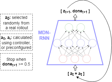
A simulation of the environment — “dream” — where the controller is used to train using the learned model only, rather than the actual environment.

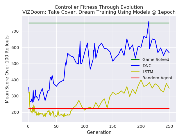
The controllers were tested in the environment throughout the generations for a 100 rollouts at each test. The results are plotted below. The MDN-DNC based controller clearly outperformed the MDN-LSTM based controller, and solved the game (achieving a mean score of 750 over 100 rollouts).

Comparison of a DNC based model versus a LSTM based model, used for training a controller in ViZDoom: Take Cover. The DNC based controller outperforms the LSTM controller.

Pommerman

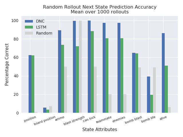
In the case of Pommerman, only the model’s predictions were used to test the capacity of the predictive model learned in a MDN-DNC and a MDN-LSTM. A controller was not trained. This was possible given that the states in Pommerman are coded as integers, rather than pixels. Thus, given [latex][s_t + a_t][/latex], the predicted state [latex][s_{t+1}][/latex] could be compared with the ground truth state from the actual game for equality, and to measure how many components of the state (position, ammo available, etc) were correctly predicted.

Here again, the MDN-DNC model outperformed the MDN-LSTM model, where both were trained exactly the same way for the same number of epochs. The MDN-DNC was more accurately able to predict the individual components of the next state given a current state and an action.

The predictive power of a DNC based model versus a LSTM based model in the Pommerman environment. The DNC based model was able to predict future states more accurately.

Conclusions

Model-based Reinforcement Learning or Evolution Strategies involve using a model of the environment when training a Reinforcement Learning or Evolution Strategies agent. In my case, the World Models approach to learn a predictive, probabilistic model of the environment in an Mixture Density Network was used. The Mixture Density Network consisted of a Differentiable Neural Computer, which output the parameters of a Gaussian mixture model that were used to sample the next state in a game. My experiments found that a model learned in a Differentiable Neural Computer outperformed a vanilla LSTM based model, on two gaming environments.

Future work should include games with long term memory dependencies, whereas with the experiments performed for this work it is hard to justify there being such dependencies in the ViZDoom: Take Cover and Pommerman environments. Other such environments would perhaps magnify the capabilities of the Differentiable Neural Computer. Also, what exactly is going on in the memory of the Differentiable Neural Computer at each timestep? It would be useful to know what it has learned, and perhaps features from the external memory of the Differentiable Neural Computer itself could be used when training a controller. For example, the Differentiable Neural Computer emits read heads, [latex]r_t[/latex], at each timestep, which are selected from the full memory, and used to produce the output (a prediction of the next state). Perhaps the contents of the read heads, or other portions of the external memory, could provide useful information of the environment if exposed directly to the controller along with the hidden state and cell state of the underlying LSTM.

Full details on this work can be found in my MSc thesis at: http://adeel.io/MSc_AI_Thesis.pdf.

References

[1] Alex Graves et al., Hybrid computing using a neural network with dynamic external memory, 2016. https://www.nature.com/articles/nature20101
[2] David Ha, Jürgen Schmidhuber, World Models, 2018. https://arxiv.org/abs/1803.10122
[3] Nikolaus Hansen, The CMA Evolution Strategy: A Tutorial, 2016. https://arxiv.org/abs/1604.00772
[4] Christopher M. Bishop, Mixture Density Networks, 1994. https://publications.aston.ac.uk/373/1/NCRG_94_004.pdf

World Models Implementation In Chainer

World Models is a framework described by
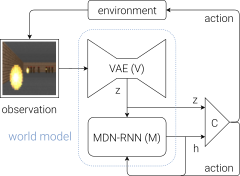
David Ha and Jürgen Schmidhuber: https://arxiv.org/abs/1803.10122. The framework aims to train an AI agent that can perform well in virtual gaming environments. World Models consists of three main components: Vision (V), Model (M), and Controller (C).

World Models Schematic

As part of my MSc Artificial Intelligence dissertation at the University of Edinburgh, I implemented World Models from the ground up in Chainer. My implementation was picked up by Chainer and tweeted:

[tweet https://twitter.com/ChainerOfficial/status/1014678023600132096]

David Ha himself also tweeted it:

[tweet https://twitter.com/hardmaru/status/1014681788680060930]

The full implementation and more details can be found at: https://github.com/AdeelMufti/WorldModels.

Mixture Density Networks in Chainer

There are excellent blog posts and guides available on Mixture Density Networks, so I will not try to replicate the effort. This post provides a quick summary, and implementation code in the Chainer deep learning framework.

In summary, Mixture Density Networks are Neural Networks that output the parameters of a Mixture Model, such as a Gaussian Mixture Model, instead of the desired output itself. The Mixture Model is then sampled from to get the final output. This is particularly useful when given a certain input, there could be multiple outputs based on some probability.

The outputs from the neural network, in the case of Gaussian Mixture Models, include a set of probabilities [latex]\alpha[/latex] (coefficients), set of means [latex]\mu[/latex], and set of standard deviations [latex]\sigma[/latex]. For example, if output is y given an x, and you choose to have 3 Gaussian mixtures, the output of your neural network would be: [latex]\alpha_1, \alpha_2, \alpha_3, \mu_1, \mu_2, \mu_2, \sigma_1, \sigma_2, \sigma_3[/latex]. The [latex]\alpha[/latex] sum to 1 and represent the probability of each mixture being the likely candidate, and the [latex]\mu[/latex] and [latex]\sigma[/latex] represent the distribution of y within the given mixture and can be used to sample y.

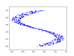
Take as a toy example consider the dataset of (x, y) coordinates represented in the graph below:

Toy dataset of (x, y) coordinates graphed.

The blue dots represent the desired y value given an x value. So at x=0.25, y could be {0, 0.5, 1} (roughly). In this case, training a neural network using Mean Squared Error to output y directly will cause the network to learn the average of the y values given x as inputs, as shown below (red dots represent y output from the neural network):

A neural network trained with Mean Squared Error produces an averaged output.

For this type of problem, a Mixture Density Network is perfectly suited. If trained properly, and sampled from enough times given all x values in the dataset, the Mixture Density Network produces the following y outputs. It better learns the distribution of the data:

A Mixture Density Network can learn the distribution of the data.

The output of the neural network is simply the number of dimensions in your output (1 in this example), times the number of desired mixtures, times 3 (the coefficient, mean, and standard distribution). In Chainer, a Linear layer can be used to output these numbers.

The loss function is essentially the negative log of the Gaussian equation multiplied by the softmax’d coefficients: [latex]-\ln\{\alpha\frac{1}{\sqrt{2\pi}\sigma}\exp{-\frac{(y-\mu)^2}{2\sigma^2}}\}[/latex], where [latex]\sum\alpha=1[/latex] [1]. This can be represented in Chainer easily as follows:

alpha = F.softmax(alpha)
density = F.sum(
    alpha *
    (1 / (np.sqrt(2 * np.pi) * F.sqrt(var))) *
    F.exp(-0.5 * F.square(y - mu) / var)
    , axis=1)
nll = -F.sum(F.log(density))

Full implementation of a Mixture Density Network in Chainer, for the toy problem shown above, can be found at: https://github.com/AdeelMufti/WorldModels/blob/master/toy/mdn.py

[1] Christopher M. Bishop, Mixture Density Networks (1994)

Changing floating point size in Chainer

The default floating point size in Chainer is 32 bit. That means for deep learning, Chainer will expect numpy.float32 for CPU or cupy.float32 for GPU under the hood, and will exit with error if the data is set at a different size.

However, there may be times you want more than 32 bits, such as when you’re getting NaN’s or inf’s in your training routine and want to troubleshoot.

Changing Chainer to use float64 is simple:

import chainer
import numpy as np
chainer.global_config.dtype = np.float64

Call this at the beginning of your program. And of course, you’ll want to make sure that the ndarray dtype’s for your data are set to float64 (as in np.array(…).astype(np.float64)) before being passed to Chainer.

Conditional GANs For Painting and Celebrity Generation

Demo: http://adeel.io/sncgan/
Code: https://github.com/AdeelMufti/SNcGAN
Paper: https://arxiv.org/abs/1903.06259

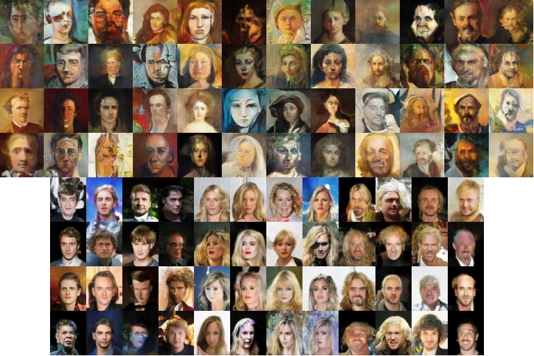
As a 4-month research project for a course at the University of Edinburgh, my group decided to use Generative Adversarial Nets to generate new paintings using the Painter by Numbers dataset. Additionally, we conditioned the paintings, allowing the generation of paintings with certain attributes (such as gender in the case of paintings of portraits). The project turned out to be a big success, and won 2nd place out of 124 other projects in a competition hosted by IBM!

The deep convolutional GAN architecture we chose for the basis of our model enforced a Lipschitz continuity constraint on the spectral norm of the weights for each layer in the discriminator, as proposed by Miyato et al. (2018). This technique, called SN-GAN by the authors, stabilizes the discriminator, allowing the generator to learn the data distribution more optimally.

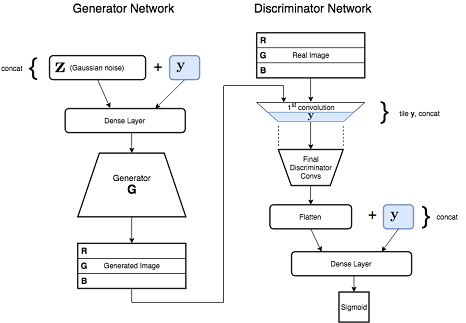
We built upon the SN-GAN architecture to add conditioning, which involved introducing a one-hot encoded y vector of supervised labels to the generator and discriminator. The y vector provides some information about the image, such as gender in the case of portrait paintings, allowing the generator to get conditioned on the label to generate the class of image specified during test time. Our contribution was a novel model which we called SN-conditional-GAN or SNcGAN, which is illustrated below.

The SNcGAN architecture. The one-hot encoded y label is introduced to the generator and discriminator.

More details can be found in our paper linked above.

After the publication of the paper, we additionally trained a SNcGAN model on the celebA dataset, allowing the generation of conditioned celebrity images.

Inspecting gradients in Chainer

Chainer is my choice of framework when it comes to implementing Neural Networks. It makes working with and trouble shooting deep learning easy.

Printing out the gradients during back propagation to inspect their values is sometimes useful in deep learning, to see if your gradients are as expected and aren’t either exploding (numbers too large) or vanishing (numbers too small). Fortunately, this is easy to do in Chainer.

Chainer provides access to the parameters in your model, and for each parameter, you can check the gradient during the back propagation step, stored in the optimizer (such as SGD or Adam). To access these, you can extend chainer.training.updaters.StandardUpdater() to additionally output the gradients, by defining your own StandardUpdater like so:

class CustomStandardUpdater(chainer.training.updaters.StandardUpdater):
    def __init__(self, train_iter, optimizer, device):
        super(CustomStandardUpdater, self).__init__(
            train_iter, optimizer, device=device)

    def update_core(self):
        super(CustomStandardUpdater, self).update_core()
        optimizer = self.get_optimizer('main')
        for name, param in optimizer.target.namedparams(include_uninit=False):
            print(name, param.grad)

In lines 9-10 you can see the parameters (weights) of your neural network being accessed through the optimizer, and for each parameter, the name and gradient is being output. This StandardUpdater can be attached to your training module as follows:

model = MyChainerModel()
optimizer.setup(model)
optimizer = chainer.optimizers.Adam()
train_iter = chainer.iterators.SerialIterator(train_dataset, batch_size=32, shuffle=True)
updater = CustomStandardUpdater(train_iter, optimizer, gpu)
trainer = training.Trainer(updater, stop_trigger=(100, 'epoch'))
trainer.run()